Did You Know :: How to Hide Rows With No Data

We have earlier discussed how to hide errors in a worksheet in this post. Today I’m going address another similar problem that is very commonly faced. There are various ways to tackle it and there is no right or wrong about it. I’m sharing what I prefer to use (because I find it very simple and easy to implement).

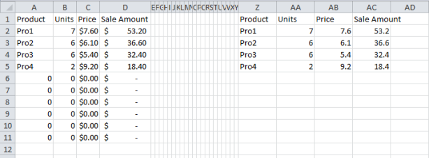
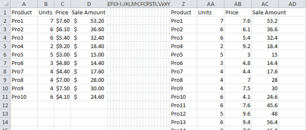
Suppose I have a data table in my dashboard that is referencing to another range. My table has 10 rows (A2:D11) that reference range Z2:AC11. As long as there is data in Z2:AC11, everything is fine.

Now suppose that I have data only till row 4. In this case, my table shows 0’s which looks ugly and I’d rather prefer those cells to be blank. How do I solve this problem?

How to Hide Errors From Worksheet Using Conditional Formatting

Today, I’m sharing a basic but nonetheless a neat trick to make your reports more presentable. I’ll take an example to illustrate my point.

I have Life Expectancy data for various countries for years 2011 and 2012.  The fourth column is calculated using data in B & C columns. The number of rows of data can change, so I have put formula in extra rows. The problem then is that the rows that don’t have data return #DIV! error in column D as below.

Did You Know ::: Automatic Subtotals (& More) :: Data List Outline

When working with a hierarchical data, most often we need to view at various levels of hierarchy. One of the ways of getting it done is using Data List Outline feature of Excel. To better demonstrate what I’m talking about, let me take an example.

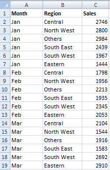
I have the following data – the first column contains the month name, the second column contains the region name and the last column has the sales.

Raw Data

Did You Know :: Finding All Objects & Controlling Object Visibility Using Selection Pane

Scenario 1 When we build dashboards in Excel, we add many objects on the worksheet. We may choose to hide some of these or make them all visible, depending on the requirement. What do you do if you want to look at all the objects on a worksheet?

Scenario 2 When you copy data from a website onto an Excel worksheet, sometime certain undesirable invisible shapes and objects also get copied over. How would you work with them if you can’t see them? Or, how would you know how many and where they are?

Did you know that you can use ‘Selection Pane‘ to do this all.

Did You Know :: Making A Workbook Read-Only

At times, when you are sharing a workbook with multiple users, you might want to make your file read-only in order to keep the users from making changes unintentionally. You can do so by making your file always open in ‘Read-Only’ mode. Once the file has been made read-only, no changes can be made to it without saving with a different name.

To make a file read-only, follow the following steps:

Did You Know :: Multiple Views of Multiple Parts of a Worksheet – Split

Some times we need to compare data located in different parts of a worksheet.
e.g. I have thousands of records in a sheet and i need to compare 1 to 25 rows with 100 to 125 rows then it is not easy to compare them in a single screen. I will have to scroll up and down again and again.
In that case splitting the worksheet into different panes makes it easy.

There are two ways to split a screen:
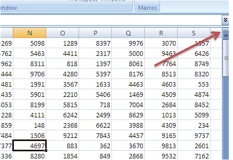
1. Using split box located at the top of the vertical scroll bar or the far right end of the horizontal scroll bar.

Just pull down that box to split the screen.

Did You Know :: Excluding Hidden Cells from SUM (and other) Formulas – SUBTOTAL

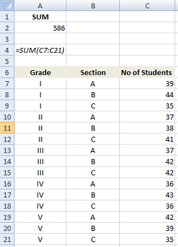
Problem Statement: I have grade-wise student numbers in column C as given below. I have written a formula in cell [A2] that sums up the total number of students in each grade.

Data

Now I want to put a filter on grade, i.e. column A, and see the total number of students in that grade in all sections. If I simply use Autofilter, it will not give the desired result.

Did You Know :: Format Comment Box

We often use cell comments to keep certain information in a spreadsheet which we may want to refer back to later. When you are creating a dashboard in Excel, and have formatted everything from a cell to a chart to look splendid, the boring-looking cell comment boxes can let your otherwise awesome report down. Did you know that you can format comment boxes just like you format a shape?

To do so, you will need to add a command to the QAT (see here how). Select ‘Shapes‘ from the list of commands and add it to the QAT.

Did You Know :: Bullet Points & Line Breaks in Excel Cells

Although Excel is a primarily a spreadsheet program, which means that it has been designed to store numbers, we often need to use some cells to store text. Also, at times we need to use ‘Word’-like features like line breaks or bullet points. Did you know that you could achieve it in Excel this way:

For bullet points – use [Alt] + 7 or [Alt] + 9 key from the numeric keypad on your keypad. The former combination will give you a filled-in bullet and latter will give you an empty bullet. In laptops where there is no dedicated keypad, use the [Fn] + [Num Lock] or [Shift] + [Num Lock] key to enable the numeric keypad and then use the shortcut for bullets.

Bullets Points in Excel Cells

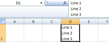
For line breaks, use [Alt] + [Enter] key

Line Breaks in Excel Cells

 

Addendum:

Using [Alt] + any number from the numeric keypad inserts the character associated with that ASCII code. In the above case, it’s the two circles.

 

 

Did You Know :: 3D Reference in Excel

A reference that refers to the same range on multiple sheets is called 3D reference. Sometimes it is very useful.

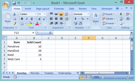
e.g.  We have a workbook that has sheets for each day(Sunday,Monday..) and a sheet named Total where we need a cumulative total.

We need to refer to the same range in each sheet. So rather than referring to each sheet range separately and then using a sum formula, there is an easy way to do it.

                                       =SUM(FirstSheet:LastSheet! Cell Address)