 We have earlier discussed how to hide errors in a worksheet in this post. Today I’m going address another similar problem that is very commonly faced. There are various ways to tackle it and there is no right or wrong about it. I’m sharing what I prefer to use (because I find it very simple and easy to implement).
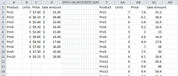
Suppose I have a data table in my dashboard that is referencing to another range. My table has 10 rows (A2:D11) that reference range Z2:AC11. As long as there is data in Z2:AC11, everything is fine.
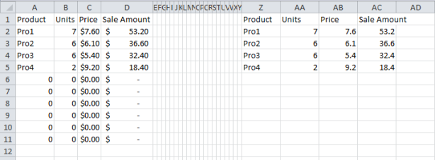
 Now suppose that I have data only till row 4. In this case, my table shows 0’s which looks ugly and I’d rather prefer those cells to be blank. How do I solve this problem?
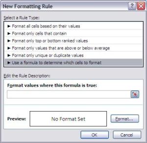
The answer is a combination of custom format and conditional formatting. I select my range A2:D11 and then add a conditional formatting rule to it (by going to Home tab -> Styles group -> Conditional Formatting -> New Rule -> Use a formula to determine which cells to format). I use this formula:
=$A2=0
Then, I click on Format -> Number tab -> Custom and use this code:
#,###;-#,###;;@
Now, click OK and you’re done.
How this works is that the formula checks if there is 0 in column A. Whenever it encounters a 0 in column A, the conditional formatting applies the custom format to the entire row. If you look at the custom format code closely, you’ll realize that what I’m essentially doing is that I’m forcing Excel not to display 0’s.
As simple as that. There may be better ways to handle this. If you have one, I’m eager to know.


